Simple Linear Regression
Fit, interpret, and check a straight-line model for a continuous outcome.

Introduction
Simple Linear Regression (SLR) is one of the most fundamental and widely used tools in epidemiology and public health research. It allows us to:
- Quantify the linear relationship between a continuous outcome and a single predictor
- Predict values of an outcome given a predictor value
- Test hypotheses about whether a predictor is associated with an outcome
- Lay the groundwork for multiple regression, which controls for confounding
In epidemiology, we frequently use SLR to model continuous outcomes such as blood pressure, BMI, cholesterol levels, or hospital length of stay as a function of age, exposure levels, or other continuous predictors.
Setup and Data
Loading BRFSS 2020 Data
We will use the Behavioral Risk Factor Surveillance System (BRFSS) 2020 data throughout this lecture. The BRFSS is a large-scale, nationally representative telephone survey conducted by the CDC that collects data on health behaviors, chronic conditions, and preventive service use among U.S. adults.
BRFSS 2020 codebook: CDC annual data page. Package documentation: brfssdata.
Data for this lecture
BRFSS 2020, loaded with the brfssdata R package. The first time you run the code below, read_brfss() downloads the 2020 survey (about 21 MB) and keeps it on your computer, so later runs read it from there. We then draw a random sample of 3,000 adults aged 18 to 80 with complete data on BMI, age, sex, education, general health, sleep, and days of poor physical health.
Install the packages once with install.packages(c("brfssdata", "janitor")).
The full BRFSS 2020 file has 401,958 respondents. We read only the seven variables this lecture needs, recode them, and draw the analytic sample. Because the code sets a seed, everyone who runs it gets the same 3,000 people.
Show the code
# Read seven BRFSS 2020 variables (CDC names; underscore names need quotes)
brfss_raw <- read_brfss(
  2020,
  vars = c("_BMI5", "_AGE80", "_SEX", "_EDUCAG", "GENHLTH", "PHYSHLTH", "SLEPTIM1")
) |>
  janitor::clean_names()

# Recode variables
brfss_slr <- brfss_raw |>
  select(bmi5, age80, sex, educag, genhlth, physhlth, sleptim1) |>
  mutate(
    bmi       = bmi5 / 100,
    age       = age80,
    sex       = factor(ifelse(sex == 1, "Male", "Female")),
    education = factor(case_when(
      educag == 1 ~ "< High school",
      educag == 2 ~ "High school graduate",
      educag == 3 ~ "Some college",
      educag == 4 ~ "College graduate"
    ), levels = c("< High school", "High school graduate",
                  "Some college", "College graduate")),
    gen_health_num = ifelse(genhlth  %in% 1:5,  genhlth,  NA_real_),
    sleep_hrs      = ifelse(sleptim1 %in% 1:24, sleptim1, NA_real_),
    phys_days      = ifelse(physhlth %in% 0:30, physhlth, NA_real_)
  )

# Select recoded variables, apply filters, drop missing, take sample
set.seed(553)
brfss_slr <- brfss_slr |>
  select(bmi, age, sex, education, gen_health_num, sleep_hrs, phys_days) |>
  filter(bmi > 14.5, bmi < 60, age >= 18, age <= 80) |>
  drop_na() |>
  slice_sample(n = 3000)

tibble(
  Metric = c("Observations", "Variables"),
  Value  = c(nrow(brfss_slr), ncol(brfss_slr))
) |>
  kable(caption = "Analytic Dataset Dimensions") |>
kable_styling(bootstrap_options = "striped", full_width = FALSE)| Metric | Value |
|---|---|
| Observations | 3000 |
| Variables | 7 |
Descriptive Statistics
Show the code
brfss_slr |>
  select(bmi, age, sleep_hrs, phys_days) |>
  summary() |>
  kable(caption = "Descriptive Statistics: Key Continuous Variables") |>
kable_styling(bootstrap_options = c("striped", "hover"), full_width = FALSE)| bmi | age | sleep_hrs | phys_days | |
|---|---|---|---|---|
| Min. :14.63 | Min. :18.00 | Min. : 1.000 | Min. : 1.00 | |
| 1st Qu.:24.32 | 1st Qu.:43.00 | 1st Qu.: 6.000 | 1st Qu.: 2.00 | |
| Median :27.89 | Median :58.00 | Median : 7.000 | Median : 6.00 | |
| Mean :29.18 | Mean :55.52 | Mean : 6.915 | Mean :11.66 | |
| 3rd Qu.:32.89 | 3rd Qu.:70.00 | 3rd Qu.: 8.000 | 3rd Qu.:20.00 | |
| Max. :59.60 | Max. :80.00 | Max. :20.000 | Max. :30.00 |
Show the code
brfss_slr |>
  select(bmi, age, sleep_hrs, sex, education) |>
  tbl_summary(
    label = list(
      bmi ~ "BMI (kg/m²)",
      age ~ "Age (years)",
      sleep_hrs ~ "Sleep (hours/night)",
      sex ~ "Sex",
      education ~ "Education"
    ),
    statistic = list(
      all_continuous() ~ "{mean} ({sd})",
      all_categorical() ~ "{n} ({p}%)"
    ),
    digits = all_continuous() ~ 1
  ) |>
  add_n() |>
  bold_labels() |>
modify_caption("**Table 1. Descriptive Statistics (BRFSS 2020, n = 3,000)**")| Characteristic | N | N = 3,0001 |
|---|---|---|
| BMI (kg/m²) | 3,000 | 29.2 (7.0) |
| Age (years) | 3,000 | 55.5 (17.4) |
| Sleep (hours/night) | 3,000 | 6.9 (1.7) |
| Sex | 3,000 | |
| Female | 1,701 (57%) | |
| Male | 1,299 (43%) | |
| Education | 3,000 | |
| < High school | 237 (7.9%) | |
| High school graduate | 796 (27%) | |
| Some college | 937 (31%) | |
| College graduate | 1,030 (34%) | |
| 1 Mean (SD); n (%) | ||
Part 1: Guided Practice
1. The Simple Linear Regression Model
1.1 What Is the Model?
Simple linear regression models the mean of a continuous outcome \(Y\) as a linear function of a single predictor \(X\):
\[Y_i = \beta_0 + \beta_1 X_i + \varepsilon_i, \quad i = 1, 2, \ldots, n\]
Where:
| Symbol | Name | Meaning |
|---|---|---|
| \(Y_i\) | Response / Outcome | Observed value for subject \(i\) (e.g., BMI) |
| \(X_i\) | Predictor / Covariate | Observed predictor for subject \(i\) (e.g., age) |
| \(\beta_0\) | Intercept | Expected value of \(Y\) when \(X = 0\) |
| \(\beta_1\) | Slope | Expected change in \(Y\) for a 1-unit increase in \(X\) |
| \(\varepsilon_i\) | Error term | Random deviation of \(Y_i\) from the regression line |
The population regression line (also called the true or theoretical regression line) describes the expected (mean) value of \(Y\) at each value of \(X\):
\[E(Y \mid X) = \mu_{Y|X} = \beta_0 + \beta_1 X\]
1.2 Key Distinction: Population vs. Sample
| Population | Sample | |
|---|---|---|
| Line | \(\beta_0 + \beta_1 X\) | \(\hat{y} = b_0 + b_1 X\) |
| Intercept | \(\beta_0\) (parameter) | \(b_0\) or \(\hat{\beta}_0\) (estimate) |
| Slope | \(\beta_1\) (parameter) | \(b_1\) or \(\hat{\beta}_1\) (estimate) |
| Error | \(\varepsilon_i\) | \(e_i = Y_i - \hat{Y}_i\) (residual) |
We use our sample to estimate the population parameters. The estimates \(b_0\) and \(b_1\) define the fitted regression line.
1.3 Visualizing the Relationship
Before fitting any model, always visualize the bivariate relationship.
Show the code
p_scatter <- ggplot(brfss_slr, aes(x = age, y = bmi)) +
  geom_point(alpha = 0.15, color = "steelblue", size = 1.2) +
  geom_smooth(method = "lm", color = "red", linewidth = 1.2, se = TRUE) +
  geom_smooth(method = "loess", color = "darkorange", linewidth = 1,
              linetype = "dashed", se = FALSE) +
  labs(
    title = "BMI vs. Age (BRFSS 2020)",
    subtitle = "Red = Linear fit | Orange dashed = LOESS smoother",
    x = "Age (years)",
    y = "BMI (kg/m²)"
  ) +
  theme_minimal(base_size = 13)

ggplotly(p_scatter)
Figure description: scatter plot of BMI against age for 3,000 adults, with points spread between about 15 and 60 kg/m² at every age. The red linear fit is nearly flat just above 29 kg/m². The orange dashed LOESS curve rises from about 24.5 kg/m² at age 18 to about 30.5 kg/m² around age 45 to 50, then falls to about 27 kg/m² by age 80.
The LOESS smoother (orange) follows the data without assuming linearity. When it closely tracks the linear fit (red), a linear model is reasonable. Departures suggest nonlinearity.
2. Assumptions of Simple Linear Regression
A useful mnemonic is LINE:
| Letter | Assumption | Description |
|---|---|---|
| L | Linearity | The relationship between \(X\) and \(E(Y)\) is linear |
| I | Independence | Observations are independent of one another |
| N | Normality | Errors \(\varepsilon_i\) are normally distributed |
| E | Equal variance | Errors have constant variance (homoscedasticity): \(\text{Var}(\varepsilon_i) = \sigma^2\) |
Formally, we assume:
\[\varepsilon_i \overset{iid}{\sim} N(0, \sigma^2)\]
This means that for any value of \(X\), the distribution of \(Y\) is:
\[Y \mid X \sim N(\beta_0 + \beta_1 X, \; \sigma^2)\]
In cross-sectional survey data like BRFSS, observations from the same household or geographic cluster may not be fully independent. We acknowledge this limitation but proceed with the standard SLR framework for pedagogical purposes.
3. Estimating the Regression Coefficients
3.1 The Method of Least Squares
We estimate \(\beta_0\) and \(\beta_1\) by finding the values \(b_0\) and \(b_1\) that minimize the sum of squared residuals (SSR):
\[SSR = \sum_{i=1}^{n}(Y_i - \hat{Y}_i)^2 = \sum_{i=1}^{n}(Y_i - b_0 - b_1 X_i)^2\]
This is called the Ordinary Least Squares (OLS) criterion. Minimizing SSR yields the closed-form solutions:
\[b_1 = \frac{\sum_{i=1}^n (X_i - \bar{X})(Y_i - \bar{Y})}{\sum_{i=1}^n (X_i - \bar{X})^2} = \frac{S_{XY}}{S_{XX}}\]
\[b_0 = \bar{Y} - b_1 \bar{X}\]
where \(\bar{X}\) and \(\bar{Y}\) are the sample means of \(X\) and \(Y\).
Under the LINE assumptions, OLS estimators are the Best Linear Unbiased Estimators (BLUE): they have the smallest variance among all linear unbiased estimators.
3.2 Fitting the Model in R
Show the code
Call:
lm(formula = bmi ~ age, data = brfss_slr)

Residuals:
    Min      1Q  Median      3Q     Max
-14.633  -4.883  -1.325   3.688  30.340

Coefficients:
             Estimate Std. Error t value Pr(>|t|)
(Intercept) 29.528231   0.427507  69.071   <2e-16 ***
age         -0.006238   0.007347  -0.849    0.396
---
Signif. codes:  0 '***' 0.001 '**' 0.01 '*' 0.05 '.' 0.1 ' ' 1

Residual standard error: 7.012 on 2998 degrees of freedom
Multiple R-squared:  0.0002404, Adjusted R-squared:  -9.312e-05
F-statistic: 0.7208 on 1 and 2998 DF,  p-value: 0.396
Show the code
# Tidy coefficient table
tidy(model_slr, conf.int = TRUE) |>
  mutate(across(where(is.numeric), ~ round(., 4))) |>
  kable(
    caption = "Simple Linear Regression: BMI ~ Age (BRFSS 2020)",
    col.names = c("Term", "Estimate", "Std. Error", "t-statistic",
                  "p-value", "95% CI Lower", "95% CI Upper"),
    align = "lrrrrrrr"
  ) |>
  kable_styling(bootstrap_options = c("striped", "hover"), full_width = FALSE) |>
row_spec(0, bold = TRUE)| Term | Estimate | Std. Error | t-statistic | p-value | 95% CI Lower | 95% CI Upper |
|---|---|---|---|---|---|---|
| (Intercept) | 29.5282 | 0.4275 | 69.0708 | 0.000 | 28.6900 | 30.3665 |
| age | -0.0062 | 0.0073 | -0.8490 | 0.396 | -0.0206 | 0.0082 |
3.3 Interpreting the Coefficients
Fitted regression equation:
\[\widehat{\text{BMI}} = 29.528 + -0.0062 \times \text{Age}\]
Intercept (\(b_0 = 29.528\)): The estimated mean BMI when age = 0. This is a mathematical artifact, because a newborn does not have an adult BMI. The intercept is not directly interpretable in this context, but is necessary to anchor the line.
Slope (\(b_1 = -0.0062\)): For each 1-year increase in age, BMI is estimated to decrease by 0.0062 kg/m², on average, holding all else constant (though there are no other variables in this simple model).
Even a small slope can be highly statistically significant with a large sample. Always consider whether the magnitude is meaningful in the real world.
3.4 Visualizing Fitted Values and Residuals
Show the code
# Augment dataset with fitted values and residuals
augmented <- augment(model_slr)

# Show a sample of fitted values and residuals
augmented |>
  select(bmi, age, .fitted, .resid) |>
  slice_head(n = 10) |>
  mutate(across(where(is.numeric), ~ round(., 3))) |>
  kable(
    caption = "First 10 Observations: Observed, Fitted, and Residual Values",
    col.names = c("Observed BMI (Y)", "Age (X)", "Fitted (Ŷ)", "Residual (e = Y − Ŷ)")
  ) |>
kable_styling(bootstrap_options = c("striped", "hover"), full_width = FALSE)| Observed BMI (Y) | Age (X) | Fitted (Ŷ) | Residual (e = Y − Ŷ) |
|---|---|---|---|
| 26.58 | 67 | 29.110 | -2.530 |
| 33.47 | 38 | 29.291 | 4.179 |
| 35.15 | 78 | 29.042 | 6.108 |
| 30.42 | 65 | 29.123 | 1.297 |
| 22.67 | 55 | 29.185 | -6.515 |
| 30.11 | 80 | 29.029 | 1.081 |
| 35.43 | 34 | 29.316 | 6.114 |
| 31.58 | 71 | 29.085 | 2.495 |
| 28.13 | 55 | 29.185 | -1.055 |
| 34.01 | 62 | 29.141 | 4.869 |
The fitted value (Ŷ) and the observed BMI (Y) are different because a person’s age does not perfectly determine their exact BMI.
- Fitted value (Ŷ): This is the predicted average BMI for anyone of a specific age, based on the trend line calculated by the model. For example, the model might calculate that the average 67-year-old has a BMI of 29.110.
- Observed BMI (Y): This is the actual, real-world BMI of a specific individual in the dataset.
- The residual or error (e = Y − Ŷ): The difference between the two is the residual or error term. The error term (εᵢ) represents the “random deviation of Yᵢ from the regression line.”
Show the code
# Select a random sample of 80 points to illustrate residuals
set.seed(42)
resid_sample <- augmented |> slice_sample(n = 80)

p_resid <- ggplot(resid_sample, aes(x = age, y = bmi)) +
  geom_segment(aes(xend = age, yend = .fitted),
               color = "tomato", alpha = 0.5, linewidth = 0.5) +
  geom_point(color = "steelblue", size = 1.8, alpha = 0.8) +
  geom_line(aes(y = .fitted), color = "black", linewidth = 1.1) +
  labs(
    title = "Residuals Illustrated on the Regression Line",
    subtitle = "Red segments = residuals (Y − Ŷ); Black line = fitted regression line",
    x = "Age (years)",
    y = "BMI (kg/m²)"
  ) +
  theme_minimal(base_size = 13)

p_resid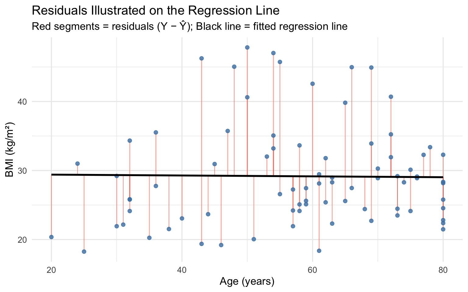
4. Partitioning Variability: ANOVA Decomposition
4.1 Sums of Squares
The total variability in \(Y\) can be decomposed into two parts:
\[\underbrace{SS_{Total}}_{Total\ variability} = \underbrace{SS_{Regression}}_{Explained\ by\ X} + \underbrace{SS_{Residual}}_{Unexplained}\]
Where:
\[SS_{Total} = \sum(Y_i - \bar{Y})^2 \qquad (df = n-1)\] \[SS_{Regression} = \sum(\hat{Y}_i - \bar{Y})^2 \qquad (df = 1)\] \[SS_{Residual} = \sum(Y_i - \hat{Y}_i)^2 \qquad (df = n-2)\]
In statistics, degrees of freedom refer to the number of independent pieces of information that are free to vary when calculating an estimate. You can think of it as the amount of “data budget” you have. Every time you estimate a parameter (like a mean or a slope), you spend one degree of freedom.
Why it’s \(n - 1\): You have \(n\) total observations. However, to calculate this variance, you first had to calculate the sample mean. Because the sum of deviations from the mean must always equal zero, knowing \(n-1\) of the deviations automatically tells you the last one. You “spent” 1 degree of freedom calculating the mean, leaving you with \(n - 1\).
Why it’s \(1\): In Simple Linear Regression, you are using exactly one predictor variable (e.g., Age) to explain the outcome (e.g., BMI). Because you are only estimating one slope parameter (\(\beta_1\)) to capture this relationship, the regression model has 1 degree of freedom. (Note: In multiple regression, this would be equal to \(k\), the number of predictor variables).
Why it’s \(n - 2\): To calculate the predicted values (\(\hat{Y}\)) and find the residuals, your model had to estimate two parameters from the data: the intercept (\(\beta_0\)) and the slope (\(\beta_1\)). Since you “spent” 2 pieces of information to create the regression line, you are left with \(n - 2\) degrees of freedom for the errors.
Show the code
# ANOVA decomposition
anova_slr <- anova(model_slr)

anova_slr |>
  kable(
    caption = "ANOVA Table: BMI ~ Age",
    digits = 3,
    col.names = c("Source", "Df", "Sum Sq", "Mean Sq", "F value", "Pr(>F)")
  ) |>
kable_styling(bootstrap_options = c("striped", "hover"), full_width = FALSE)| Source | Df | Sum Sq | Mean Sq | F value | Pr(>F) |
|---|---|---|---|---|---|
| age | 1 | 35.438 | 35.438 | 0.721 | 0.396 |
| Residuals | 2998 | 147400.214 | 49.166 | NA | NA |
4.2 Mean Squared Error (MSE) and \(\hat{\sigma}\)
The Mean Squared Error estimates the variance of the error term:
\[MSE = \frac{SS_{Residual}}{n - 2} = \hat{\sigma}^2\]
The Residual Standard Error \(\hat{\sigma} = \sqrt{MSE}\) is in the same units as \(Y\) and tells us the typical prediction error of the model.
Show the code
n <- nrow(brfss_slr)
ss_resid <- sum(augmented$.resid^2)
mse <- ss_resid / (n - 2)
sigma_hat <- sqrt(mse)

tibble(
  Quantity = c("SS Residual", "MSE (σ̂²)", "Residual Std. Error (σ̂)"),
  Value    = c(round(ss_resid, 2), round(mse, 3), round(sigma_hat, 3)),
  Units    = c("", "", "kg/m²")
) |>
  kable(caption = "Model Error Estimates") |>
kable_styling(bootstrap_options = "striped", full_width = FALSE)| Quantity | Value | Units |
|---|---|---|
| SS Residual | 147400.210 | |
| MSE (σ̂²) | 49.166 | |
| Residual Std. Error (σ̂) | 7.012 | kg/m² |
On average, our model’s predictions are off by about 7.01 BMI units.
5. The Coefficient of Determination: R²
5.1 Definition and Interpretation
\(R^2\) measures the proportion of total variability in \(Y\) explained by the linear regression on \(X\):
\[R^2 = \frac{SS_{Regression}}{SS_{Total}} = 1 - \frac{SS_{Residual}}{SS_{Total}}\]
\(R^2\) ranges from 0 to 1:
- \(R^2 = 0\): \(X\) explains none of the variability in \(Y\)
- \(R^2 = 1\): \(X\) explains all variability in \(Y\) (perfect fit)
Show the code
# Extract R-squared from model
r_sq <- summary(model_slr)$r.squared
adj_r_sq <- summary(model_slr)$adj.r.squared

tibble(
  Metric = c("R²", "Adjusted R²", "Variance Explained"),
  Value  = c(
    round(r_sq, 4),
    round(adj_r_sq, 4),
    paste0(round(r_sq * 100, 2), "%")
  )
) |>
  kable(caption = "R² and Adjusted R²") |>
kable_styling(bootstrap_options = "striped", full_width = FALSE)| Metric | Value |
|---|---|
| R² | 2e-04 |
| Adjusted R² | -1e-04 |
| Variance Explained | 0.02% |
5.2 Relationship Between R² and Pearson’s r
For simple linear regression:
\[R^2 = r^2\]
where \(r\) is the Pearson correlation coefficient between \(X\) and \(Y\).
Show the code
r_pearson <- cor(brfss_slr$age, brfss_slr$bmi)
tibble(
  Quantity   = c("Pearson r", "r² (from Pearson)", "R² (from model)", "r² = R²?"),
  Value      = c(
    round(r_pearson, 4),
    round(r_pearson^2, 4),
    round(r_sq, 4),
    as.character(round(r_pearson^2, 4) == round(r_sq, 4))
  )
) |>
  kable(caption = "Pearson r vs. R² from Model") |>
kable_styling(bootstrap_options = "striped", full_width = FALSE)| Quantity | Value |
|---|---|
| Pearson r | -0.0155 |
| r² (from Pearson) | 2e-04 |
| R² (from model) | 2e-04 |
| r² = R²? | TRUE |
A low \(R^2\) does not mean the regression is useless. In epidemiology, outcomes are influenced by many unmeasured factors, so \(R^2\) values of 0.05 to 0.20 can still yield scientifically meaningful and statistically significant estimates.
6. Hypothesis Testing
6.1 Testing the Slope: Is There a Linear Association?
The most important hypothesis test in SLR is:
\[H_0: \beta_1 = 0 \quad \text{(no linear relationship between X and Y)}\] \[H_A: \beta_1 \neq 0 \quad \text{(there is a linear relationship)}\]
Test statistic:
\[t = \frac{b_1 - 0}{SE(b_1)} \sim t_{n-2} \quad \text{under } H_0\]
Where:
\[SE(b_1) = \frac{\hat{\sigma}}{\sqrt{\sum(X_i - \bar{X})^2}} = \frac{\hat{\sigma}}{\sqrt{S_{XX}}}\]
Show the code
# Extract slope test statistics
slope_test <- tidy(model_slr, conf.int = TRUE) |> filter(term == "age")

tibble(
  Quantity = c("Slope (b₁)", "SE(b₁)", "t-statistic",
               "Degrees of freedom", "p-value", "95% CI Lower", "95% CI Upper"),
  Value    = c(
    round(slope_test$estimate, 4),
    round(slope_test$std.error, 4),
    round(slope_test$statistic, 3),
    n - 2,
    format.pval(slope_test$p.value, digits = 3),
    round(slope_test$conf.low, 4),
    round(slope_test$conf.high, 4)
  )
) |>
  kable(caption = "t-Test for the Slope (H₀: β₁ = 0)") |>
kable_styling(bootstrap_options = "striped", full_width = FALSE)| Quantity | Value |
|---|---|
| Slope (b₁) | -0.0062 |
| SE(b₁) | 0.0073 |
| t-statistic | -0.849 |
| Degrees of freedom | 2998 |
| p-value | 0.396 |
| 95% CI Lower | -0.0206 |
| 95% CI Upper | 0.0082 |
Decision: With p = 0.396, we fail to reject \(H_0\) at the \(\alpha = 0.05\) level. The data do not provide statistically significant evidence of a linear association between age and BMI, and the 95% confidence interval for the slope includes zero.
6.2 The F-Test: Overall Model Significance
The F-test evaluates whether the overall model (i.e., all predictors together) explains a statistically significant portion of the variability in \(Y\). For simple linear regression with one predictor, the F-test is equivalent to the t-test for the slope (\(F = t^2\)).
\[F = \frac{MS_{Regression}}{MS_{Residual}} \sim F_{1,\, n-2} \quad \text{under } H_0\]
- The numerator: This represents the amount of variability in the data that your model successfully explains.
- The denominator: This represents the “leftover” or unexplained variability (the errors).
When your model does a good job of predicting the outcome, the explained variance goes up, and the unexplained variance goes down. This makes the resulting F-statistic larger. What a higher F-statistic means for your results:
- Lower p-value: A larger F-statistic pushes the p-value closer to zero.
- Statistical significance: If the p-value drops below your alpha level (usually 0.05), you can reject the null hypothesis. It gives you confidence that your overall model actually has some predictive power, rather than just capturing random noise.
Show the code
f_stat <- summary(model_slr)$fstatistic
f_value <- f_stat[1]
df1 <- f_stat[2]
df2 <- f_stat[3]
p_f <- pf(f_value, df1, df2, lower.tail = FALSE)

tibble(
  Quantity = c("F-statistic", "df (numerator)", "df (denominator)",
               "p-value", "Verification: t²", "Verification: F"),
  Value    = c(
    round(f_value, 3),
    df1,
    df2,
    format.pval(p_f, digits = 3),
    round(slope_test$statistic^2, 3),
    round(f_value, 3)
  )
) |>
  kable(caption = "F-Test for Overall Model Significance") |>
kable_styling(bootstrap_options = "striped", full_width = FALSE)| Quantity | Value |
|---|---|
| F-statistic | 0.721 |
| df (numerator) | 1 |
| df (denominator) | 2998 |
| p-value | 0.396 |
| Verification: t² | 0.721 |
| Verification: F | 0.721 |
6.3 Confidence Interval for the Slope
A 95% CI for \(\beta_1\) is:
\[b_1 \pm t_{n-2, \, 0.025} \times SE(b_1)\]
Show the code
t_crit <- qt(0.975, df = n - 2)
ci_lower <- slope_test$estimate - t_crit * slope_test$std.error
ci_upper <- slope_test$estimate + t_crit * slope_test$std.error

tibble(
  Bound = c("95% CI Lower", "95% CI Upper"),
  Value = c(round(ci_lower, 4), round(ci_upper, 4)),
  Units = c("kg/m² per year", "kg/m² per year")
) |>
  kable(caption = "95% Confidence Interval for β₁ (manually computed)") |>
kable_styling(bootstrap_options = "striped", full_width = FALSE)| Bound | Value | Units |
|---|---|---|
| 95% CI Lower | -0.0206 | kg/m² per year |
| 95% CI Upper | 0.0082 | kg/m² per year |
7. Confidence Intervals and Prediction Intervals
7.1 Estimating the Mean Response (Confidence Interval)
A confidence interval for the mean response \(E(Y \mid X = x^*)\) gives a range of plausible values for the population mean of \(Y\) at a specific value \(x^*\):
\[\hat{Y}^* \pm t_{n-2, \, \alpha/2} \times SE(\hat{Y}^*)\]
Where:
\[SE(\hat{Y}^*) = \hat{\sigma}\sqrt{\frac{1}{n} + \frac{(x^* - \bar{X})^2}{S_{XX}}}\]
7.2 Predicting a Single Observation (Prediction Interval)
A prediction interval gives a range for a single new observation \(Y^*_{new}\) at \(X = x^*\). It is always wider than the confidence interval because it accounts for both the uncertainty in \(E(Y)\) and the individual variability around the mean:
\[\hat{Y}^* \pm t_{n-2, \, \alpha/2} \times SE_{pred}\]
Where:
\[SE_{pred} = \hat{\sigma}\sqrt{1 + \frac{1}{n} + \frac{(x^* - \bar{X})^2}{S_{XX}}}\]
Show the code
# Compute CI and PI at specific age values
new_ages <- data.frame(age = c(25, 35, 45, 55, 65, 75))

ci_pred <- predict(model_slr, newdata = new_ages, interval = "confidence") |>
  as.data.frame() |>
  rename(Fitted = fit, CI_Lower = lwr, CI_Upper = upr)

pi_pred <- predict(model_slr, newdata = new_ages, interval = "prediction") |>
  as.data.frame() |>
  rename(PI_Lower = lwr, PI_Upper = upr) |>
  select(-fit)

results_table <- bind_cols(new_ages, ci_pred, pi_pred) |>
  mutate(across(where(is.numeric), ~ round(., 2)))

results_table |>
  kable(
    caption = "Fitted Values, 95% Confidence Intervals, and Prediction Intervals by Age",
    col.names = c("Age", "Fitted BMI", "CI Lower", "CI Upper", "PI Lower", "PI Upper")
  ) |>
  kable_styling(bootstrap_options = c("striped", "hover"), full_width = FALSE) |>
add_header_above(c(" " = 2, "95% CI for Mean" = 2, "95% PI for Individual" = 2))| Age | Fitted BMI | CI Lower | CI Upper | PI Lower | PI Upper |
|---|---|---|---|---|---|
| 25 | 29.37 | 28.87 | 29.88 | 15.61 | 43.13 |
| 35 | 29.31 | 28.92 | 29.70 | 15.56 | 43.06 |
| 45 | 29.25 | 28.95 | 29.54 | 15.50 | 43.00 |
| 55 | 29.19 | 28.93 | 29.44 | 15.43 | 42.94 |
| 65 | 29.12 | 28.84 | 29.41 | 15.37 | 42.87 |
| 75 | 29.06 | 28.68 | 29.44 | 15.31 | 42.81 |
Show the code
# Generate CI and PI across the full age range
age_grid <- data.frame(age = seq(18, 80, length.out = 200))

ci_band <- predict(model_slr, newdata = age_grid, interval = "confidence") |>
  as.data.frame() |>
  bind_cols(age_grid)

pi_band <- predict(model_slr, newdata = age_grid, interval = "prediction") |>
  as.data.frame() |>
  bind_cols(age_grid)

p_ci_pi <- ggplot() +
  geom_point(data = brfss_slr, aes(x = age, y = bmi),
             alpha = 0.10, color = "steelblue", size = 1) +
  geom_ribbon(data = pi_band, aes(x = age, ymin = lwr, ymax = upr),
              fill = "lightblue", alpha = 0.3) +
  geom_ribbon(data = ci_band, aes(x = age, ymin = lwr, ymax = upr),
              fill = "steelblue", alpha = 0.4) +
  geom_line(data = ci_band, aes(x = age, y = fit),
            color = "red", linewidth = 1.2) +
  labs(
    title = "Simple Linear Regression: BMI ~ Age",
    subtitle = "Dark band = 95% CI for mean response | Light band = 95% PI for individual observation",
    x = "Age (years)",
    y = "BMI (kg/m²)",
    caption = "BRFSS 2020, n = 3,000"
  ) +
  theme_minimal(base_size = 13)

p_ci_pi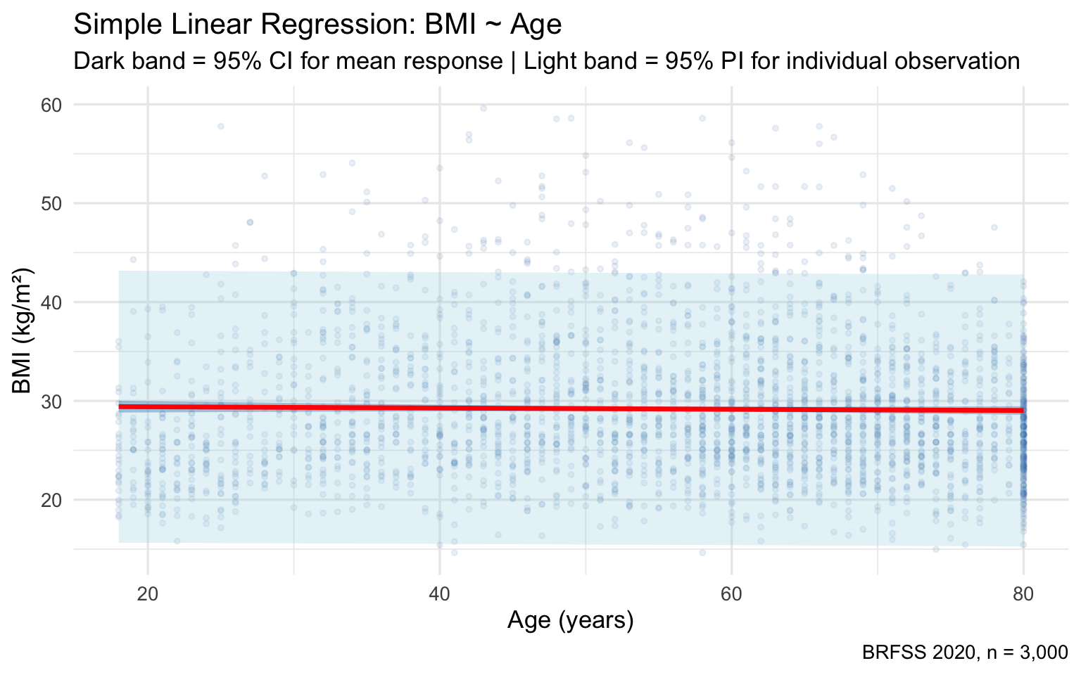
If you want to estimate the average BMI for all 45-year-olds in the population, use the confidence interval. If you want to predict the BMI of a specific new 45-year-old patient, use the prediction interval.
8. Checking Model Assumptions (Diagnostics)
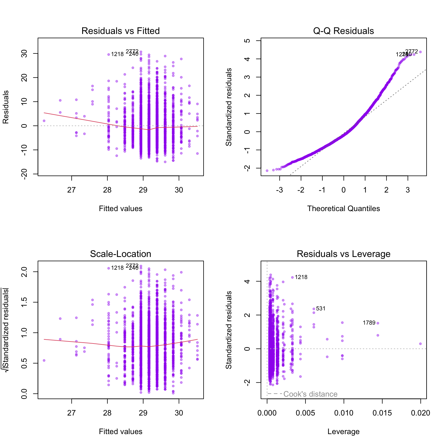
Fitting a regression model is not enough; we must verify that the LINE assumptions are reasonably met. We do this through residual diagnostics.
8.1 The Four Standard Diagnostic Plots
Show the code
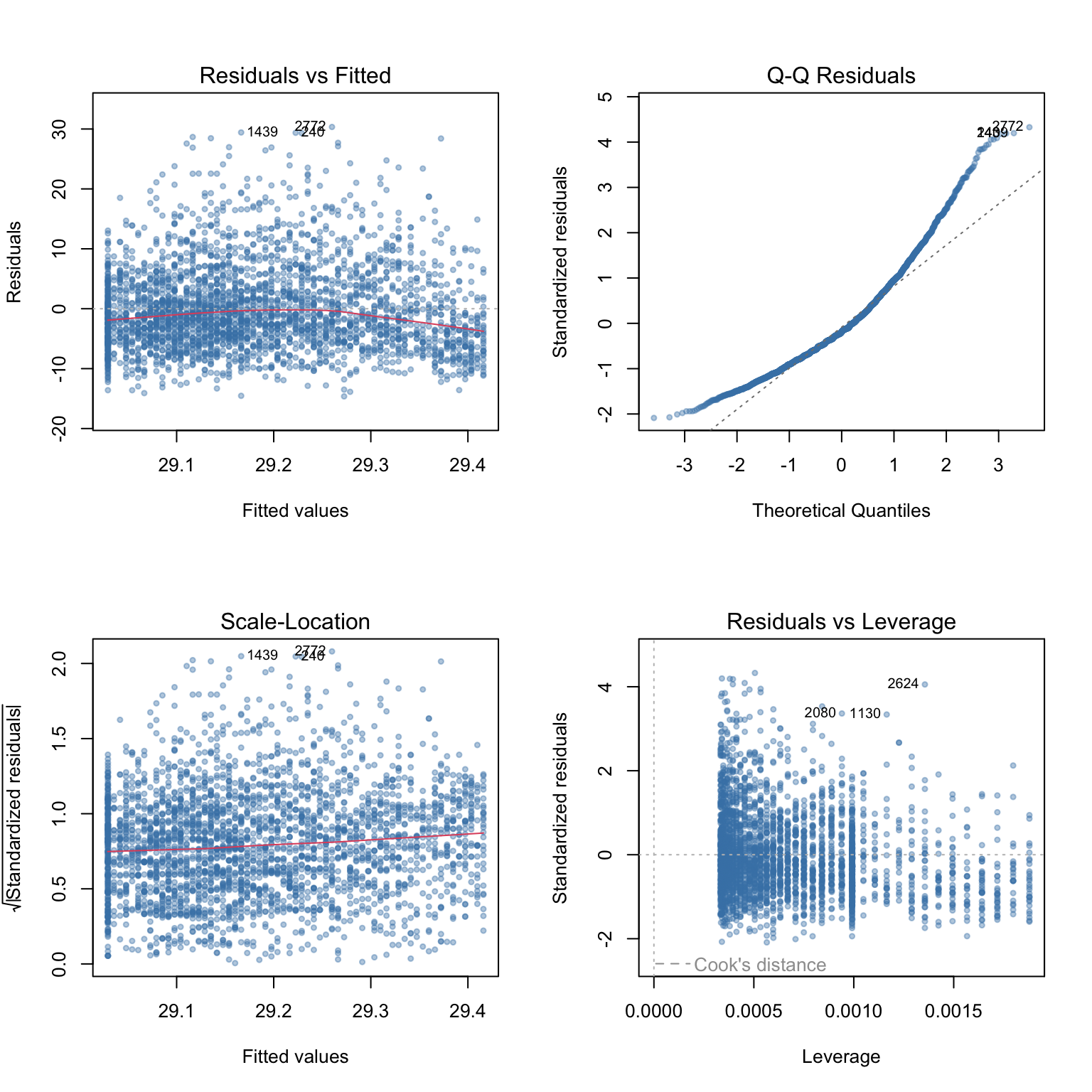
Interpreting each plot:
1. Residuals vs. Fitted: Checks linearity and equal variance. We want a horizontal red line and random scatter with no pattern. A “fan shape” (spread increasing with fitted values) indicates heteroscedasticity.
2. Normal Q-Q Plot: Checks normality of residuals. Points should fall approximately along the 45° reference line. Heavy tails or S-curves suggest non-normality.
3. Scale-Location (Spread-Location): Another check for equal variance (homoscedasticity). The square root of standardized residuals is plotted against fitted values. A flat line indicates constant variance.
4. Residuals vs. Leverage: Identifies influential observations using Cook’s distance. Points in the upper or lower right corner (beyond the dashed lines) have high influence.
8.2 Residuals vs. Predictor
The Residuals vs. Predictor plot is a visual diagnostic tool used to check if your data meets the core assumptions of Simple Linear Regression, specifically Linearity and Equal Variance (Homoscedasticity).
Show the code
p_resid_x <- ggplot(augmented, aes(x = age, y = .resid)) +
  geom_point(alpha = 0.15, color = "steelblue", size = 1) +
  geom_hline(yintercept = 0, color = "red", linewidth = 1) +
  geom_smooth(method = "loess", color = "orange", se = FALSE, linewidth = 1) +
  labs(
    title = "Residuals vs. Age",
    subtitle = "Should show no pattern: random scatter around zero",
    x = "Age (years)",
    y = "Residuals"
  ) +
  theme_minimal(base_size = 13)

p_resid_x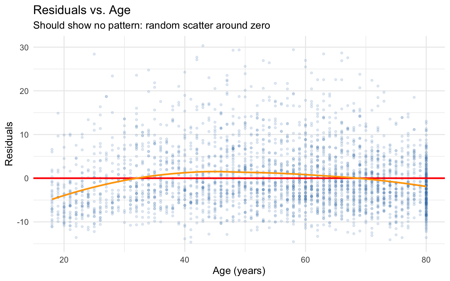
- Y-axis (Residuals): The errors from your model. This is how far off each person’s actual BMI was from the model’s predicted BMI.
- X-axis (Age): Your predictor variable. (In Simple Linear Regression with only one predictor, this plot looks identical in shape to the “Residuals vs. Fitted” plot.)
What do the lines mean?
- The red line: This is a flat, horizontal line at exactly zero. If the model predicted a person’s BMI perfectly, their point would land exactly on this line.
- The orange line (LOESS smoother): This is a moving average of the residuals. It helps your eye track the overall trend of the errors across different ages.
Interpretation
The orange line stays fairly close to the red line, though there is a very slight curve downwards at the extreme ends of the age range. The vertical spread of the points looks relatively consistent across the ages. Overall, it doesn’t show any severe violations of linearity or equal variance, though there is a lot of random scatter (which aligns with the very low \(R^2\) value we saw earlier).
8.3 Histogram and Q-Q Plot of Residuals
Show the code
p_hist <- ggplot(augmented, aes(x = .resid)) +
  geom_histogram(aes(y = after_stat(density)), bins = 40,
                 fill = "steelblue", color = "white", alpha = 0.8) +
  geom_density(color = "red", linewidth = 1) +
  stat_function(fun = dnorm,
                args = list(mean = mean(augmented$.resid),
                            sd = sd(augmented$.resid)),
                color = "black", linetype = "dashed", linewidth = 1) +
  labs(
    title = "Distribution of Residuals",
    subtitle = "Red = kernel density | Black dashed = normal distribution",
    x = "Residuals",
    y = "Density"
  ) +
  theme_minimal(base_size = 13)

p_hist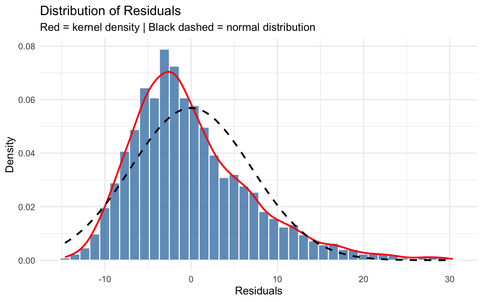
Show the code
# ggplot version of QQ plot
p_qq <- ggplot(augmented, aes(sample = .resid)) +
  stat_qq(color = "steelblue", alpha = 0.3, size = 1) +
  stat_qq_line(color = "red", linewidth = 1) +
  labs(
    title = "Normal Q-Q Plot of Residuals",
    subtitle = "Points should lie on the red line if residuals are normally distributed",
    x = "Theoretical Quantiles",
    y = "Sample Quantiles"
  ) +
  theme_minimal(base_size = 13)

p_qq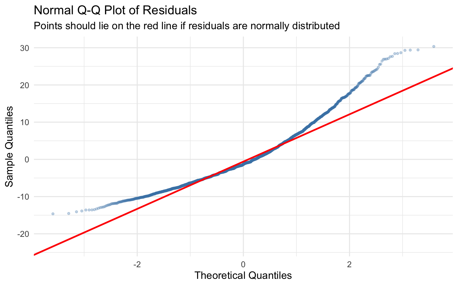
8.4 Identifying Influential Observations
Show the code
# Cook's distance
augmented <- augmented |>
  mutate(
    obs_num = row_number(),
    cooks_d = cooks.distance(model_slr),
    influential = ifelse(cooks_d > 4 / n, "Potentially influential", "Not influential")
  )

n_influential <- sum(augmented$cooks_d > 4 / n)

p_cooks <- ggplot(augmented, aes(x = obs_num, y = cooks_d, color = influential)) +
  geom_point(alpha = 0.6, size = 1.2) +
  geom_hline(yintercept = 4 / n, linetype = "dashed",
             color = "red", linewidth = 1) +
  scale_color_manual(values = c("Potentially influential" = "tomato",
                                "Not influential" = "steelblue")) +
  labs(
    title = "Cook's Distance",
    subtitle = paste0("Dashed line = 4/n threshold | ",
                      n_influential, " potentially influential observations"),
    x = "Observation Number",
    y = "Cook's Distance",
    color = ""
  ) +
  theme_minimal(base_size = 13) +
  theme(legend.position = "top")

p_cooks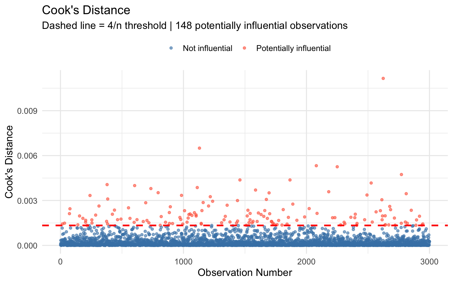
9. A Second Example: Sleep and BMI
To reinforce the concepts, let’s fit a second SLR model examining the association between hours of sleep and BMI.
Show the code
p_sleep <- ggplot(brfss_slr, aes(x = sleep_hrs, y = bmi)) +
  geom_jitter(alpha = 0.15, color = "purple", width = 0.15, height = 0) +
  geom_smooth(method = "lm", color = "darkred", linewidth = 1.2, se = TRUE) +
  labs(
    title = "BMI vs. Nightly Sleep Hours (BRFSS 2020)",
    x = "Average Hours of Sleep per Night",
    y = "BMI (kg/m²)"
  ) +
  theme_minimal(base_size = 13)

p_sleep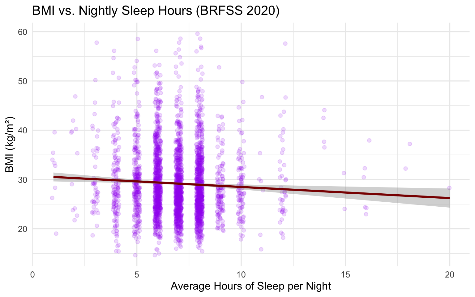
Show the code
model_sleep <- lm(bmi ~ sleep_hrs, data = brfss_slr)

tidy(model_sleep, conf.int = TRUE) |>
  mutate(across(where(is.numeric), ~ round(., 4))) |>
  kable(
    caption = "SLR: BMI ~ Hours of Sleep per Night",
    col.names = c("Term", "Estimate", "Std. Error", "t-statistic",
                  "p-value", "95% CI Lower", "95% CI Upper")
  ) |>
kable_styling(bootstrap_options = c("striped", "hover"), full_width = FALSE)| Term | Estimate | Std. Error | t-statistic | p-value | 95% CI Lower | 95% CI Upper |
|---|---|---|---|---|---|---|
| (Intercept) | 30.7419 | 0.534 | 57.5683 | 0.0000 | 29.6948 | 31.7890 |
| sleep_hrs | -0.2256 | 0.075 | -3.0087 | 0.0026 | -0.3726 | -0.0786 |
Show the code
| Metric | Value |
|---|---|
| Slope (b₁) | -0.2256 |
| R² | 0.0030 |
Interpretation: Each additional hour of sleep per night is associated with a change of -0.2256 kg/m² in BMI, on average. The direction of this association is negative (more sleep → lower BMI). The model explains 0.3% of variability in BMI. While statistically significant, the effect size is modest, underscoring the multifactorial nature of BMI.
10. Does BMI Really Decrease with Age? Adding a Quadratic Term
Our linear model estimated a negative slope for age: older adults have, on average, slightly lower BMI. But is that the full story? Cross-sectional data can show a decline at older ages due to survivorship bias: people with very high BMI may die before reaching old age, leaving a healthier-looking older sample. There may also be a genuine nonlinear pattern (BMI rises through middle age, then declines in later life).
We can test this by including an age² term in the model:
\[\widehat{\text{BMI}} = b_0 + b_1 \cdot \text{Age} + b_2 \cdot \text{Age}^2\]
This is still a linear regression model (linear in the coefficients), even though it is nonlinear in the predictor. It allows the slope to change across the range of age.
Show the code
# Add age-squared term
brfss_slr <- brfss_slr |>
  mutate(age2 = age^2)

# Fit quadratic model
model_quad <- lm(bmi ~ age + age2, data = brfss_slr)

tidy(model_quad, conf.int = TRUE) |>
  mutate(across(where(is.numeric), ~ round(., 5))) |>
  kable(
    caption = "Quadratic Model: BMI ~ Age + Age²",
    col.names = c("Term", "Estimate", "Std. Error", "t-statistic",
                  "p-value", "95% CI Lower", "95% CI Upper")
  ) |>
kable_styling(bootstrap_options = c("striped", "hover"), full_width = FALSE)| Term | Estimate | Std. Error | t-statistic | p-value | 95% CI Lower | 95% CI Upper |
|---|---|---|---|---|---|---|
| (Intercept) | 18.54178 | 1.08095 | 17.15329 | 0 | 16.42230 | 20.66125 |
| age | 0.47435 | 0.04418 | 10.73772 | 0 | 0.38773 | 0.56096 |
| age2 | -0.00464 | 0.00042 | -11.02651 | 0 | -0.00546 | -0.00381 |
Show the code
# Compare linear vs. quadratic model
tibble(
  Model       = c("Linear: BMI ~ Age", "Quadratic: BMI ~ Age + Age²"),
  R_squared   = c(
    round(summary(model_slr)$r.squared, 4),
    round(summary(model_quad)$r.squared, 4)
  ),
  Adj_R2      = c(
    round(summary(model_slr)$adj.r.squared, 4),
    round(summary(model_quad)$adj.r.squared, 4)
  ),
  AIC         = c(round(AIC(model_slr), 1), round(AIC(model_quad), 1))
) |>
  kable(
    caption = "Model Comparison: Linear vs. Quadratic",
    col.names = c("Model", "R²", "Adj. R²", "AIC")
  ) |>
  kable_styling(bootstrap_options = c("striped", "hover"), full_width = FALSE) |>
  row_spec(which.min(c(AIC(model_slr), AIC(model_quad))),
bold = TRUE, background = "#d4edda", color = "#1f2d3a")| Model | R² | Adj. R² | AIC |
|---|---|---|---|
| Linear: BMI ~ Age | 0.0002 | -0.0001 | 20203.2 |
| Quadratic: BMI ~ Age + Age² | 0.0392 | 0.0386 | 20085.9 |
Show the code
# Generate predicted values from both models
age_seq <- data.frame(age = seq(18, 80, length.out = 300)) |>
  mutate(age2 = age^2)

pred_linear <- predict(model_slr, newdata = age_seq)
pred_quad   <- predict(model_quad, newdata = age_seq)

pred_df <- age_seq |>
  mutate(
    linear    = pred_linear,
    quadratic = pred_quad
  ) |>
  pivot_longer(cols = c(linear, quadratic),
               names_to = "Model", values_to = "Predicted_BMI")

ggplot() +
  geom_point(data = brfss_slr, aes(x = age, y = bmi),
             alpha = 0.10, color = "steelblue", size = 1) +
  geom_line(data = pred_df, aes(x = age, y = Predicted_BMI, color = Model),
            linewidth = 1.3) +
  scale_color_manual(
    values = c("linear" = "red", "quadratic" = "darkorange"),
    labels = c("linear" = "Linear fit", "quadratic" = "Quadratic fit (Age + Age²)")
  ) +
  labs(
    title = "BMI vs. Age: Linear vs. Quadratic Model",
    subtitle = "Does BMI rise then fall with age, or decline monotonically?",
    x = "Age (years)",
    y = "BMI (kg/m²)",
    color = "Model"
  ) +
  theme_minimal(base_size = 13) +
  theme(legend.position = "top")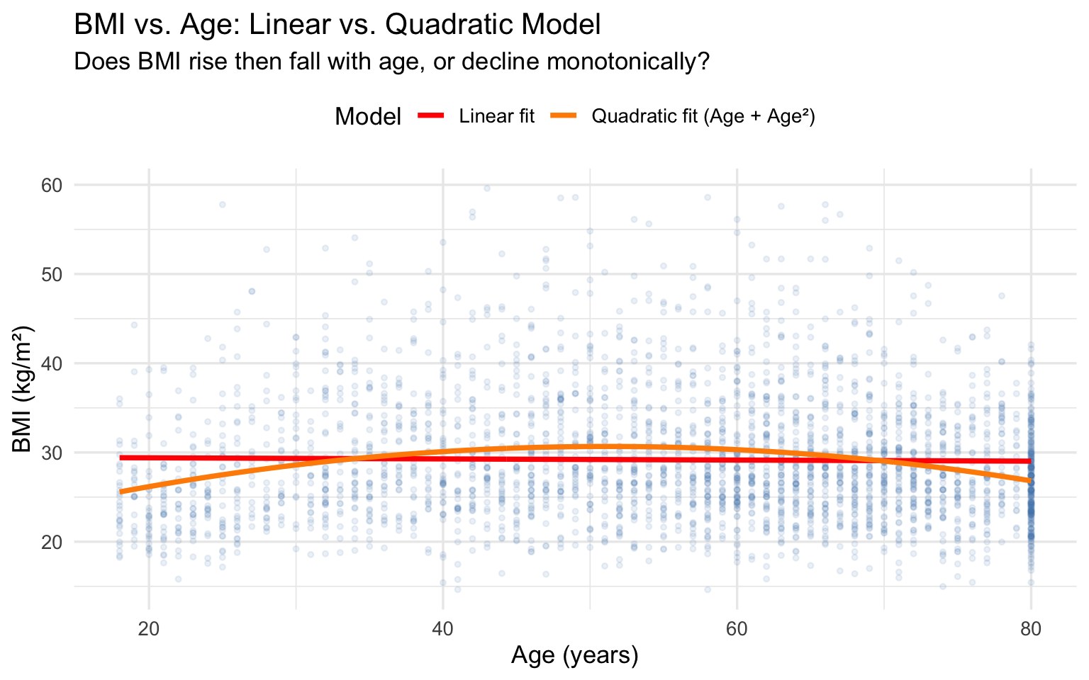
If the coefficient on Age² is negative and statistically significant, the fitted curve is an inverted U: BMI peaks at some middle age and declines thereafter. Extract the peak using \(\text{Age}^* = -b_1 / (2 b_2)\). A positive Age² coefficient would indicate a U-shape (BMI lowest in middle age).
Show the code
b1_q <- coef(model_quad)["age"]
b2_q <- coef(model_quad)["age2"]

peak_age <- -b1_q / (2 * b2_q)

tibble(
  Quantity = c("b₁ (Age)", "b₂ (Age²)", "Peak / Trough Age (-b₁ / 2b₂)"),
  Value    = c(round(b1_q, 5), round(b2_q, 6), round(peak_age, 1))
) |>
  kable(caption = "Quadratic Model Coefficients and Implied Turning Point") |>
kable_styling(bootstrap_options = "striped", full_width = FALSE)| Quantity | Value |
|---|---|
| b₁ (Age) | 0.474350 |
| b₂ (Age²) | -0.004635 |
| Peak / Trough Age (-b₁ / 2b₂) | 51.200000 |
Even if the quadratic model fits better statistically, be cautious about causal interpretation. The cross-sectional pattern reflects cohort differences in BMI trajectories, not necessarily the aging process within any individual. Survivorship bias (heavier individuals dying earlier) can make the quadratic term appear significant in cross-sectional data.
11. Summary of Key Formulas
| Quantity | Formula |
|---|---|
| Slope | \(b_1 = S_{XY} / S_{XX}\) |
| Intercept | \(b_0 = \bar{Y} - b_1 \bar{X}\) |
| SSTotal | \(\sum(Y_i - \bar{Y})^2\) |
| SSRegression | \(\sum(\hat{Y}_i - \bar{Y})^2\) |
| SSResidual | \(\sum(Y_i - \hat{Y}_i)^2\) |
| MSE | \(SS_{Residual} / (n-2)\) |
| \(R^2\) | \(SS_{Reg} / SS_{Total}\) |
| \(SE(b_1)\) | \(\hat{\sigma}/\sqrt{S_{XX}}\) |
| t-statistic | \(b_1 / SE(b_1)\) |
| 95% CI for \(\beta_1\) | \(b_1 \pm t_{n-2, 0.025} \cdot SE(b_1)\) |
Part 2: Lab Activity
Overview
In this lab, you will apply Simple Linear Regression to the BRFSS 2020 dataset using a different outcome variable: number of days of poor physical health in the past 30 days (phys_days). You will model it as a continuous outcome predicted by BMI.
Research Question: Is BMI associated with the number of days of poor physical health among U.S. adults?
Setup Instructions
The lab uses the same 3,000 adults as the lecture. Put the code below at the top of your lab .qmd. If you have not used brfssdata before, install it first with install.packages(c("brfssdata", "janitor")); the first run downloads BRFSS 2020 once, and later runs read it from your computer.
Show the code
# Load packages
library(tidyverse)
library(brfssdata)
library(knitr)
library(kableExtra)
library(broom)

# Read and recode BRFSS 2020 (same steps as the lecture)
brfss_lab <- read_brfss(
  2020,
  vars = c("_BMI5", "_AGE80", "_SEX", "_EDUCAG", "GENHLTH", "PHYSHLTH", "SLEPTIM1")
) |>
  janitor::clean_names() |>
  mutate(
    bmi       = bmi5 / 100,
    age       = age80,
    sex       = factor(ifelse(sex == 1, "Male", "Female")),
    education = factor(case_when(
      educag == 1 ~ "< High school",
      educag == 2 ~ "High school graduate",
      educag == 3 ~ "Some college",
      educag == 4 ~ "College graduate"
    ), levels = c("< High school", "High school graduate",
                  "Some college", "College graduate")),
    gen_health_num = ifelse(genhlth  %in% 1:5,  genhlth,  NA_real_),
    sleep_hrs      = ifelse(sleptim1 %in% 1:24, sleptim1, NA_real_),
    phys_days      = ifelse(physhlth %in% 0:30, physhlth, NA_real_)
  )

# Draw the same sample as the lecture, then keep the lab variables
set.seed(553)
brfss_lab <- brfss_lab |>
  select(bmi, age, sex, education, gen_health_num, sleep_hrs, phys_days) |>
  filter(bmi > 14.5, bmi < 60, age >= 18, age <= 80) |>
  drop_na() |>
  slice_sample(n = 3000) |>
  select(bmi, age, sex, phys_days, sleep_hrs)
Task 1: Explore the Variables (15 points)
Show the code
# (a) Create a summary table of phys_days and bmi


# (b) Create a histogram of phys_days, then describe the distribution


# (c) Create a scatter plot of phys_days (Y) vs bmi (X)
Questions:
What is the mean and standard deviation of
phys_days? Ofbmi? What do you notice about the distribution ofphys_days?Based on the scatter plot, does the relationship between BMI and poor physical health days appear to be linear? Are there any obvious outliers?
Task 2: Fit and Interpret the SLR Model (20 points)
Show the code
# (a) Fit the SLR model: phys_days ~ bmi


# (b) Display a tidy coefficient table with 95% CIs


# (c) Extract and report: slope, intercept, t-statistic, p-value
Questions:
Write the fitted regression equation in the form \(\hat{Y} = b_0 + b_1 X\).
Interpret the slope (\(b_1\)) in context. What does it mean in plain English?
Is the intercept (\(b_0\)) interpretable in this context? Why or why not?
Is the association statistically significant at \(\alpha = 0.05\)? State the null hypothesis, test statistic, and p-value.
Task 3: ANOVA Decomposition and R² (15 points)
Show the code
# (a) Display the ANOVA table


# (b) Compute and report SSTotal, SSRegression, and SSResidual


# (c) Compute R² two ways: from the model object and from the SS decomposition
Questions:
Fill in the ANOVA table components: \(SS_{Total}\), \(SS_{Regression}\), \(SS_{Residual}\), \(df\), and \(F\)-statistic.
What is the \(R^2\) value? Interpret it in plain English.
What does this \(R^2\) tell you about how well BMI alone explains variation in poor physical health days? What might explain the remaining variation?
Task 4: Confidence and Prediction Intervals (20 points)
Show the code
# (a) Calculate the fitted value and 95% CI for a person with BMI = 25


# (b) Calculate the 95% prediction interval for a person with BMI = 25


# (c) Plot the regression line with both the CI band and PI band
Questions:
For someone with a BMI of 25, what is the estimated mean number of poor physical health days? What is the 95% confidence interval for this mean?
If a specific new person has a BMI of 25, what is the 95% prediction interval for their number of poor physical health days?
Explain in your own words why the prediction interval is wider than the confidence interval. When would you use each one in practice?
Task 5: Residual Diagnostics (20 points)
Show the code
# (a) Produce the four standard diagnostic plots (use par(mfrow = c(2,2)) and plot())


# (b) Create a residuals vs. fitted plot using ggplot


# (c) Create a normal Q-Q plot of residuals using ggplot


# (d) Create a Cook's distance plot
Questions:
Examine the Residuals vs. Fitted plot. Is there evidence of nonlinearity or heteroscedasticity? Describe what you see.
Examine the Q-Q plot. Are the residuals approximately normal? What do departures from normality in this context suggest about the distribution of
phys_days?Are there any influential observations (Cook’s D > 4/n)? How many? What would you do about them?
Overall, do the LINE assumptions appear to be met? Which assumption(s) may be most problematic for this model, and why? (Hint: think about the nature of the outcome variable.)
Task 6: Testing a Different Predictor (10 points)
Now fit a second SLR model using age as the predictor of phys_days instead of BMI.
Show the code
# (a) Fit SLR: phys_days ~ age


# (b) Display results and compare to the BMI model


# (c) Which predictor has the stronger association? Compare R² values.
Questions:
How does the association between age and poor physical health days compare to the BMI association in terms of direction, magnitude, and statistical significance?
Compare the \(R^2\) values of the two models. Which predictor explains more variability in
phys_days?Based on these two simple models, what is your overall conclusion about predictors of poor physical health days? What are the limitations of using simple linear regression for this outcome?
Submission Instructions
Upload two files to the Brightspace assignment: your completed .qmd (or .Rmd) file and the rendered HTML file. The HTML must open on its own, with its figures inside it. In a .qmd, put this in the YAML header at the top of the file before you render:
format:
  html:
    embed-resources: true
An .Rmd that uses output: html_document does this by default.
Your file must render without errors. Make sure all code chunks produce visible output and all questions are answered in complete sentences below each code chunk.
Due: Before the next class session.
R version 4.6.1 (2026-06-24)
Platform: aarch64-apple-darwin23
Running under: macOS Golden Gate 27.2

Matrix products: default
BLAS:   ~/.uvr/r-versions/4.6.1/lib/libRblas.0.dylib
LAPACK: ~/.uvr/r-versions/4.6.1/lib/libRlapack.dylib;  LAPACK version 3.12.1

locale:
[1] en_US.UTF-8/en_US.UTF-8/en_US.UTF-8/C/en_US.UTF-8/en_US.UTF-8

time zone: America/New_York
tzcode source: internal

attached base packages:
[1] stats     graphics  grDevices utils     datasets  methods   base

other attached packages:
 [1] gtsummary_2.6.1  ggeffects_2.3.2  broom_1.0.13     plotly_4.12.1
 [5] kableExtra_1.4.1 knitr_1.52       brfssdata_0.1.1  lubridate_1.9.5
 [9] forcats_1.0.1    stringr_1.6.0    dplyr_1.2.1      purrr_1.2.2
[13] readr_2.2.0      tidyr_1.3.2      tibble_3.3.1     ggplot2_4.0.3
[17] tidyverse_2.0.0

loaded via a namespace (and not attached):
 [1] gtable_0.3.6        xfun_0.62           htmlwidgets_1.6.4
 [4] insight_1.7.0       lattice_0.23-1      tzdb_0.5.0
 [7] crosstalk_1.2.2     vctrs_0.7.3         tools_4.6.1
[10] generics_0.1.4      stats4_4.6.1        pkgconfig_2.0.3
[13] Matrix_1.7-6        data.table_1.18.6.1 RColorBrewer_1.1-3
[16] S7_0.2.2            gt_1.4.0            lifecycle_1.0.5
[19] compiler_4.6.1      farver_2.1.2        textshaping_1.0.5
[22] janitor_2.2.1       mitools_2.7         snakecase_0.11.1
[25] survey_4.5          litedown_1.0        sass_0.4.10
[28] htmltools_0.5.9     yaml_2.3.12         pillar_1.11.1
[31] nlme_3.1-172        tidyselect_1.2.1    digest_0.6.39
[34] stringi_1.8.9       duckdb_2.0.0        labeling_0.4.3
[37] splines_4.6.1       fastmap_1.2.0       grid_4.6.1
[40] cli_3.6.6           magrittr_2.0.5      base64enc_0.1-6
[43] cards_0.9.0         survival_3.8-12     withr_3.0.3
[46] scales_1.4.0        backports_1.5.1     timechange_0.4.0
[49] rmarkdown_2.32      httr_1.4.9          otel_0.2.0
[52] srvyr_1.3.1         hms_1.1.4           evaluate_1.0.5
[55] viridisLite_0.4.3   mgcv_1.9-4          markdown_2.1
[58] rlang_1.3.0         Rcpp_1.1.2          glue_1.8.1
[61] DBI_1.3.0           xml2_1.6.0          svglite_2.2.2
[64] rstudioapi_0.19.0   jsonlite_2.0.0      R6_2.6.1
[67] fs_2.1.0            systemfonts_1.3.2